University of Washington · Composite materials education
Design, test, simulate
and manufacture composites
Define a fiber-reinforced material, conduct virtual tests, simulate processing and load the laminate to first-ply failure.
Educational simulations and illustrative material models. AI-generated images, not to scale.
1Pick a fiber
+ 8552 epoxyHexcel 8552 Epoxy resin · 0% voids
2Set ply directions
Always 100%Fiber, volume fraction and layup
Select a fiber, its volume fraction and the ply percentages, then compare stiffness, strength, mass and cost. Every design is a 3 mm, 32-ply symmetric, balanced laminate.
Set your design on the left, then select Compare designs.
32 plies · 3 mm total · symmetric & balanced
Your design · hover to preview, click to load
Specific stiffness & strength
Per unit density · log scalesDirectional stiffness
Stiffness in x versus yEstimated tensile strength
First-ply failure in x versus y · log scalesMass & raw material cost
One marker per fiber · independent of ply directionReading the plots & model assumptions
Marker shape identifies the fiber. Color identifies the layup: more than 50% of plies at 0°, 90° or ±45° forms a dominated group; the rest are mixed. Shaded envelopes group the selected fiber’s sampled layups. They do not represent additional designs. At zero fiber content, ply directions are physically equivalent.
The main map uses specific stiffness E/ρ in MN·m/kg and specific strength σ/ρ in kN·m/kg. Choose x or y loading above that map. Both axes on this map, and both strength axes, use logarithmic scales so weak and strong directions remain readable. Axes are fixed for all five fibers and 0–70% fiber volume.
All five fibers are compared at the same selected fiber volume fraction, using Hexcel 8552 Epoxy resin and zero voids. Every panel is 3 mm thick with 32 equal-thickness, symmetric and balanced 0°/90°/±45° plies. Layup changes mechanical response, while mass and raw material cost stay fixed at a given fiber and volume fraction.
Stiffness uses classical laminate theory. Estimated tensile strengths use the constituent-based maximum-strain model in separate uniaxial x and y tensile tests. First-ply failure is initiation, not ultimate strength. Fully cured, room-temperature estimates. Bending, buckling, compression, progressive damage, manufacturing cost and waste are outside this study.
This study is independent of the shared material until you select Open in Laminate Builder. Hover or focus a marker for a graphical layup and every property; click to load the design. Arrow keys explore points. A ring marks the same selected design in all four plots.
Define your specimen
The test and all five reference specimens have the same thickness and test settings.
After the first run, the signals follow your changes.
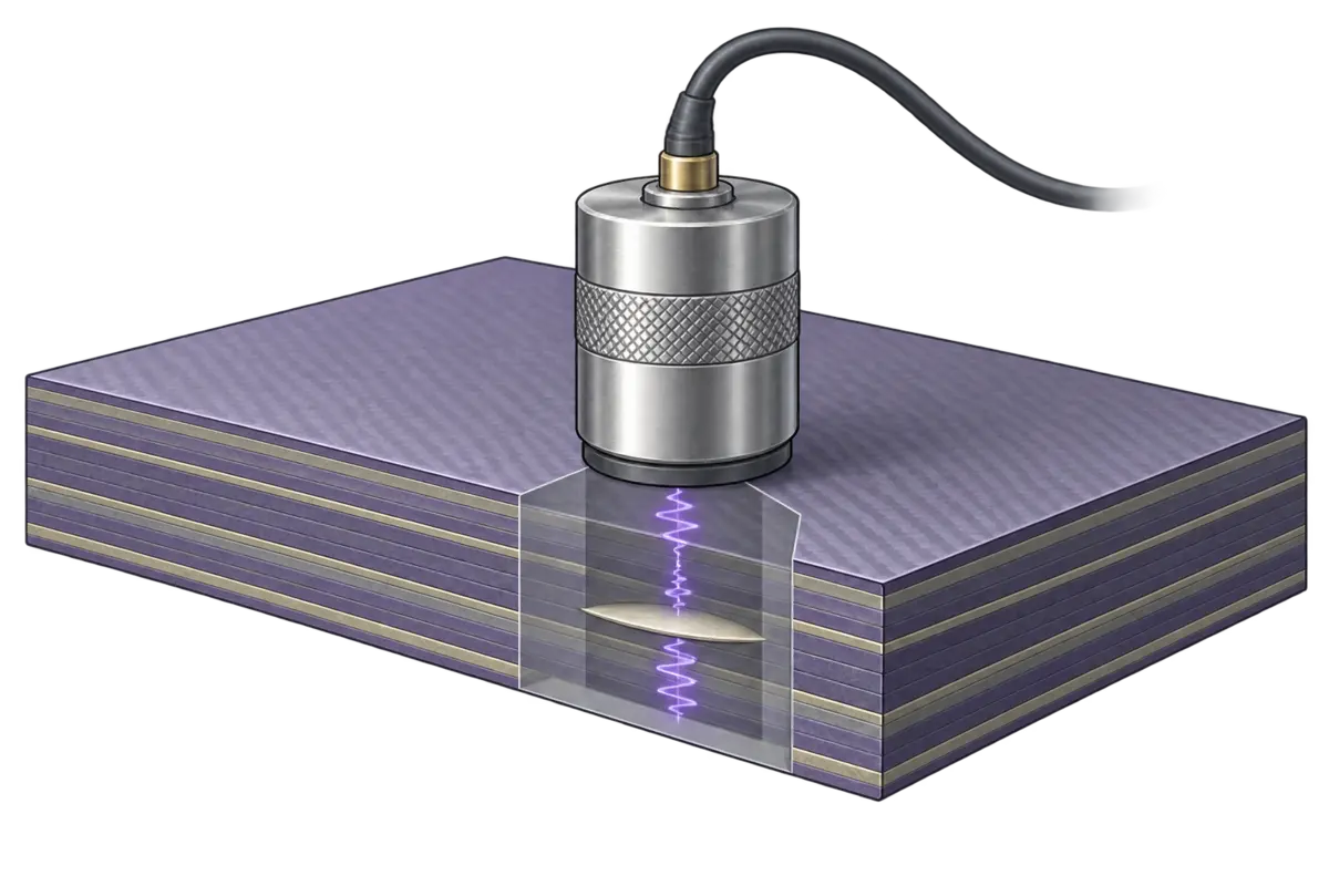
Porosity and delamination detection
Compare reference specimens with 0, 2, 4, 6 and 8% porosity. Porosity attenuates the backwall echo; a delamination returns an earlier echo.
An illustrative reference set for learning, rather than measured calibration data.
Compare the echoes
Model and reference assumptions
These are synthetic echo envelopes for a nominal 2.5 MHz test, with fixed amplitude scaling, coupling and acoustic velocity (3 mm/µs). All reference specimens have the same thickness. Porosity is a separate teaching input; Material Builder does not supply measured acoustic properties.
Pressure amplitude follows A = A₀ exp(−2αd), with d in mm and α = 0.02 + 0.0125p in Np/mm, where p is porosity in percent (0–8). The slope is illustrative, not fitted to measured 8552 data. Real calibration depends on material, layup, frequency, void morphology, thickness and coupling.
The delamination is one planar reflector at the selected depth, with nominal pressure reflection coefficient r = 0.9. Its earlier echo is attenuated over its own round trip; the backwall echo is multiplied by 1 − r². Multiple reverberations, scattering noise and full wave propagation are omitted. Echoes may overlap when an interface is close to a surface.
A weak backwall echo alone cannot distinguish porosity from a delamination or poor coupling. A specimen with an extra interface echo should not be assigned a porosity by this amplitude calibration.
Background: Johnston et al., thermal and ultrasonic evaluation of porosity; reference calibration. These sources support the teaching concepts, not the numerical coefficients used here.
Test a lamina
The same stiffness and strain limits are used in Laminate Builder and Mechanical Tests.
Compare 0°, 45° and 90°. The curve ends at estimated first failure.
Stiffness and strength versus fiber angle
A unidirectional ply is stiff and strong along the fibers and weak across them. Load it off-axis and see how the modulus and first-failure stress fall with angle.
Select Test the lamina, then drag the fiber angle.
Thermal resistance
R = 1/h for the air and L/k for each layer, in 10⁻³ m²K/W (part k at 100 °C, uncured). The largest resistance limits how fast heat gets in during heat-up, and how fast exotherm heat gets out.
The result is checked against these limits everywhere in the part.
4Try a cycleChoose a starting point
Temperature and degree of cure through the thickness
Circulating hot air heats the part and tool. Run the cycle to explore thermal lag, reaction heat and cure through the part.
Adjust the setup on the left, then select Run.
Material state through the part
Local part temperature and cure · αgel = 0.5 · Glassy band: Tg ≥ T + 25 °C (course convention).
Overshoot is the most the part runs above the air; lag is the most it runs below (heat-up and holds only). Max heating rate is the largest dT/dt the part reaches at that point, from the solved temperatures at every time step.
1Define constituents and fractions
Maximum combined fiber fraction: 70%.
2Explore assumptionsComposition, failure and constituent data
Composition by volume and mass
Estimated ply failure properties
Calculated from the constituents, fiber content and voids. Both virtual tests use these limits.
| Failure mode | Strength MPa | Strain % |
|---|
Model equations
Fiber and resin data
Shared with Burn-off Test, DSC Test, Rheology Test, Cure Simulation, Laminate Builder and Mechanical Tests.
Constituents and volume fractions
Choose fibers and their volume fractions. See how composition changes stiffness, strength, thermal properties and raw material cost.
Adjust the setup on the left, then select Run.
All properties & plot choices
Use + to add a plot. Selected plots have a filled dot.
Equations
Composition
Voids sit in the resin, so Vm = 1 − Vf − Vv, and the share of the resin that is void is p = Vv / (Vm + Vv).
ρ = Vf ρf + Vm ρm wf = Vf ρf / ρ wr = 1 − wf
Elastic properties
Porous resin: Em′ = Em (1 − p)², Gm′ = Em (1 − p)² / [2 (1 + νm)]
E1 = Vf Ef1 + (1 − Vf) Em′ (rule of mixtures)
P / Pm = (1 + ξ η Vf) / (1 − η Vf), η = (Pf/Pm − 1) / (Pf/Pm + ξ) (Halpin–Tsai)
with P = E2, ξ = 2 (fiber Ef2) and P = G12, ξ = 1 (fiber Gf12).
ν12 = Vf νf + (1 − Vf) νm
Heat
Resin conductivity km = 0.148 + 3.43×10⁻⁴ T + 0.0607 α (W/m·K, T in °C), reduced by voids as km′ = km (1 − p) / (1 + p/2) (Maxwell).
k11 = Vf kf1 + (1 − Vf) km′
k33 = km′ [1 − 2√(Vf/π) + (1/B) (π − (4/s) tan⁻¹( s / (1 + B √(Vf/π)) ))], B = 2 (km′/kf2 − 1), s = √(1 − B² Vf/π) (Springer–Tsai)
If resin and transverse fiber conductivities are equal, k33 equals that same conductivity.
cp = (Vf ρf cpf + Vm ρm cpm) / ρ
1D cure uses k33 and cp at every time step, at the local temperature and degree of cure; the resin cpm also changes as the resin vitrifies.
Cure
Heat of reaction of part: Hpart = HR wr (J/g)
Volumetric heat of reaction of part: Hvol = HR ρm Vm / 1000 (MJ/m³)
HR = 600 J/g of uncured Hexcel 8552 Epoxy resin; ρm is resin density in kg/m³. Part values include the fiber and resin fractions. Only the resin releases reaction heat.
Two fibers and cost
A mix uses fiber properties averaged by volume (by mass for cp). Constituent cost per kg = Σ wi ci, with wi = Vi ρi / ρ for each fiber and the resin. Voids add no mass or cost. Fixed teaching prices: E-glass $2/kg, S-glass $15/kg, Kevlar 49 $20/kg, AS4 carbon $25/kg, IM7 carbon $40/kg and Hexcel 8552 Epoxy resin $10/kg. These nominal values illustrate relative costs, rather than supplier quotations. This estimate excludes prepreg conversion and manufacturing costs.
1Layup
Layup
Enter layup as text
Use commas, spaces or slashes.
2Ply thickness or areal weight
All fibers combined, excluding resin.
Uses the fiber volume fraction and composition from Material.
Mass per ply by constituent
3Try a layupChoose a starting stack
Every ply uses the material defined in Material.
Stacking sequence and laminate stiffness
Arrange ply directions and define the thickness. Then see the stack, directional stiffness and equivalent laminate properties.
Adjust the setup on the left, then select Run.
The ply stack
Stiffness by direction
Membrane Young’s modulusABD matrices & full properties
The main plot and cards show membrane properties with bending restrained (κ = 0), calculated from A. The free-to-bend response (M = 0) includes extension–bending coupling and can be softer for an asymmetric layup. Compare both below.
Ply coordinates & conventions
Ply 1 starts at z = −h/2. The bottom is z = +h/2. Positive angles are counterclockwise from x when viewed from above. Engineering shear: ε(z) = ε⁰ + zκ.
Equations and assumptions
Classical laminate theory: linear elastic, plane stress, perfectly bonded plies. Ply E₁, E₂, G₁₂ and ν₁₂ come from Material. These elastic constants are fixed estimates, independent of the cure simulation. Transverse shear deformation is omitted.
ν₂₁ = ν₁₂ E₂/E₁; Q₁₁ = E₁/(1 − ν₁₂ν₂₁); Q₂₂ = E₂/(1 − ν₁₂ν₂₁); Q₁₂ = ν₁₂ E₂/(1 − ν₁₂ν₂₁); Q₆₆ = G₁₂.
Q̄ is the plane-stress ply stiffness rotated by each ply angle using engineering shear.
A = Σ Q̄ₖ (zₖ − zₖ₋₁); B = ½ Σ Q̄ₖ (zₖ² − zₖ₋₁²); D = ⅓ Σ Q̄ₖ (zₖ³ − zₖ₋₁³).
{N; M} = [A B; B D] {ε⁰; κ}. Main display: aₘ = A⁻¹; Eₓ = 1/(h aₘ₁₁), Eᵧ = 1/(h aₘ₂₂), Gₓᵧ = 1/(h aₘ₆₆), νₓᵧ = −aₘ₁₂/aₘ₁₁. These are membrane properties with κ = 0.
For the free-to-bend properties (M = 0), use the upper-left block a of ABD⁻¹ in place of aₘ. For B = 0 the two definitions coincide. With the same material and orientation fractions, membrane properties are independent of stacking order. Bending properties and coupling can still change.
Bending: Eₓᵇ = 12/(h³ d₁₁), Eᵧᵇ = 12/(h³ d₂₂), Gₓᵧᵇ = 12/(h³ d₆₆), νₓᵧᵇ = −d₁₂/d₁₁.
Per ply: FAW = t Vf Σ qiρi; FAWi = t Vf qiρi; resin areal mass = t (1 − Vf − Vv)ρr. Here t is in mm, densities in kg/m³ and areal masses in g/m². qi is each fiber’s volume share within the fibers. Total ply areal mass includes resin; voids add no mass.
Mass/area = ρh; constituent cost/area = (mass/area) × material cost/kg. Laminate thickness is reported here; the independent 1D cure thickness remains editable.
Reference: NASA RP-1351, Basic Mechanics of Laminated Composite Plates.
1Three-point bend testLoad–displacement and first failure
Use the current material and layup. The curve ends at estimated first-ply failure.
2Tensile testStress–strain and first failure
Report tensile modulus, stress and strain at first-ply failure. The stress–strain response does not require specimen dimensions.
Uses the same material and layup as the bending test.
Three-point bending and tension to first-ply failure
Load the laminate in three-point bending or tension. Follow the load–displacement curve and see which ply reaches its failure strain first.
Adjust the setup on the left, then select Run.
The bending specimen
Elastic loadingLoad–displacement
Equations & assumptions
Room-temperature, linear elastic response from the shared Material and Laminate definitions, independent of the simulated cure state. Loading is along laminate x. Five strain limits are calculated in Material from constituent properties, fiber volume and void fraction. Curves stop when any ply first reaches a longitudinal, transverse or engineering-shear limit. No progressive damage or ultimate laminate failure is predicted.
Tension: Nx = σ h; Ny = Nxy = 0; M = 0; [ε⁰; κ] = ABD⁻¹ [N; M].
Tensile Eₓ allows free bending (M = 0). Geometry is unnecessary for the stress–strain curve. The specimen graphic is schematic; scaled extension and contraction illustrate the elastic response.
Bending: I = bh³/12; EI = Eₓᵇ I; P = 48EI δ/L³.
Bending at midspan: Mx = PL/(4b); My = Mxy = 0; N = 0. Nominal flexural stress = 3PL/(2bh²).
At both faces of every ply: ε(z) = ε⁰ + zκ. ε₁ = m²εx + n²εy + mnγxy; ε₂ = n²εx + m²εy − mnγxy; γ₁₂ = −2mnεx + 2mnεy + (m² − n²)γxy.
For each component, divide its strain magnitude by the matching tension, compression or engineering-shear limit. The maximum ratio over all ply faces is the failure index. Scale the applied load until that index is 1. In bending, all faces are checked at midspan, where the moment is largest. First-ply failure is an initiation estimate. Transverse cracking or shear yielding need not cause ultimate laminate failure. The constituent model and its fixed teaching assumptions are listed in Material.
Equivalent narrow-beam bending uses Eₓᵇ from the laminate compliance with N = 0 and transverse/twisting moments free. The drawing shows longitudinal deflection only. Small deflections, ideal simple supports and perfect bonding are assumed. Transverse shear deformation, contact indentation, grip effects, damage and geometric nonlinearity are omitted. Nominal flexural stress is not the stress in an individual ply.
References: ASTM D3039, tensile properties; ASTM D7264, flexural properties; Roylance, beam displacements. This is a teaching simulation, not a complete implementation of either ASTM procedure.
Predicted first failure
Strain details
1Specimen
Enter your measurements. Each stage removes one constituent; the residue is what is left in the crucible.
| T °C | Mass after g | Removed | ρ g/cm³ |
|---|---|---|---|
Leave unused stage rows empty. Results update as you type.
Staged burn-off in air
Heat the specimen in air, in steps. Each constituent burns at its own temperature (epoxy 350 °C, Kevlar 450 °C, AS4 550 °C, IM7 600 °C), so each hold removes one of them. Glass does not burn and is left in the crucible. Weigh after every hold, then use the masses, densities and the original volume to find Vf, Vm and Vv.
Select Start burn-off test, or switch to My lab data to analyze your own measurements.
Show the calculation
Method, equations and assumptions
Removed mass mi = m(before) − m(after). Volume vi = mi/ρi. Volume fraction Vi = vi/V₀ and weight fraction Wi = mi/m₀. Void fraction Vv = 1 − ΣVi. Composite density ρc = m₀/V₀. Always divide by the original bulk volume V₀, never by the volume of the residue.
Burn temperatures in air: epoxy 350 °C, Kevlar 49 450 °C, AS4 carbon 550 °C, IM7 carbon 600 °C; glass fiber does not burn. The furnace holds at each burn temperature in turn, so each hold removes one constituent while everything with a higher burn temperature survives. Glass is always the final residue. Because AS4 and IM7 burn at different temperatures they can be separated; two glass fibers cannot, so a glass/glass hybrid gives one combined glass volume fraction. Each hold runs to constant mass with complete, selective removal and no char or sizing residue. When two constituents leave in the same hold (two glass grades stay together as the residue), the notebook uses their combined density.
In the virtual test the balance reads to 0.001 g and V₀ to 0.01 cm³, as in a lab, so the recovered void fraction differs slightly from the value set in Material Builder. Small voids come from the difference of large numbers, so measurement resolution matters.
In practice: ASTM D2584 (ignition loss) for glass composites, ASTM D3171 (matrix digestion) for carbon composites, and ASTM D2734 for void content from density. Background: McDonough et al., carbon/glass hybrid constituent and void content (NIST, 2004).
1Sample
The resin comes from your shared material.
Properties
2Temperature program
Each hold starts at its temperature, with no heat-up ramp.
A small resin sample that follows the set temperature exactly, so there is no thermal lag.
3Try a cycleChoose a starting point
Reaction heat flow during cure
A resin sample and reference follow the same temperature program. The plotted signal is reaction heat flow per gram of resin.
Define a program, then select Run DSC test.
1Resin and material stateHexcel 8552 Epoxy resin
Hexcel 8552 Epoxy resin
The resin model is shared with DSC and Cure Simulation.
About the model
Viscosity is the Hexcel 8552 Epoxy resin flow model before gelation. Material state uses cure and Tg. The post-gel illustrations are qualitative; storage modulus, loss modulus and frequency dependence are not calculated.
Gelation: α = 0.5. The timeline follows the course vitrification convention, Tg ≥ T + 25 °C. Glass transition is a broad, timescale-dependent change; these bands show the teaching classification.
Model source: 8552 material characterization · NIAR/NCAMP reference. The gelation factor multiplies both temperature terms. The app uses the MSE 475 gel point α = 0.5 for gelation and for the viscosity divergence; the reference fit used 0.545. Full citation and adaptations: About & license → Models and assumptions.
2Temperature cycle
3Try a cycleOne hold, or cool and reheat
Viscosity and gelation
Heating lowers the viscosity; cure raises it until gelation (α = 0.5) ends liquid flow.
Define a cycle, then select Run rheology test.
Gelation: α = 0.5 · Glassy band: Tg ≥ T + 25 °C (course convention).
Properties
Columns: temperature (°C), heat flow (W/g) and, ideally, time. Header lines are skipped.
Data columns and units
Explore the heat under the curve
Open a dynamic DSC test file on the left. The residual heat under the exotherm gives the degree of cure of the sample before the test. Not sure of the format? .
How the degree of cure is calculated
1Design space
2Try a studyChoose a starting point
Cure-cycle processing window
Vary one or two settings. Each combination is simulated and checked against the peak-temperature and degree-of-cure specifications.
Adjust the setup on the left, then select Run.
Select results to include. Download a self-contained report that you can print or save as PDF.
Each run is compared at one point: the mid-plane of a laminate, or the facesheet point with the largest lag in a sandwich.
From constituents to laminate response
Material Builder defines the constituents, fiber volume fraction and void content. Characterization, process simulation and the laminate stiffness and failure analyses all use this one material definition.
Use, cite and license
Free to use, share and adapt with credit.
Cite as
Zobeiry, N. (2026). UW Composites Analysis: interactive composite materials lab [Web application]. University of Washington. https://doi.org/10.5281/zenodo.23431546
BibTeX
@software{zobeiry_uw_composites_analysis_2026,
  author    = {Zobeiry, Navid},
  title     = {{UW Composites Analysis}: interactive composite materials lab},
  year      = {2026},
  publisher = {University of Washington},
  doi       = {10.5281/zenodo.23431546},
  url       = {https://composites.uw.edu/analysis/}
}Full license text and third-party notices
Software: MIT License. Original educational text and diagrams: Creative Commons Attribution 4.0 International (CC BY 4.0). Credit the author, link to the source and license, and indicate changes when sharing adaptations.
Third-party libraries, fonts, referenced publications and institutional names or marks retain their own terms.
Content license notice · Third-party notices
Full MIT software license
MIT License

Copyright (c) 2026 Navid Zobeiry

Permission is hereby granted, free of charge, to any person obtaining a copy
of this software and associated documentation files (the "Software"), to deal
in the Software without restriction, including without limitation the rights
to use, copy, modify, merge, publish, distribute, sublicense, and/or sell
copies of the Software, and to permit persons to whom the Software is
furnished to do so, subject to the following conditions:

The above copyright notice and this permission notice shall be included in all
copies or substantial portions of the Software.

THE SOFTWARE IS PROVIDED "AS IS", WITHOUT WARRANTY OF ANY KIND, EXPRESS OR
IMPLIED, INCLUDING BUT NOT LIMITED TO THE WARRANTIES OF MERCHANTABILITY,
FITNESS FOR A PARTICULAR PURPOSE AND NONINFRINGEMENT. IN NO EVENT SHALL THE
AUTHORS OR COPYRIGHT HOLDERS BE LIABLE FOR ANY CLAIM, DAMAGES OR OTHER
LIABILITY, WHETHER IN AN ACTION OF CONTRACT, TORT OR OTHERWISE, ARISING FROM,
OUT OF OR IN CONNECTION WITH THE SOFTWARE OR THE USE OR OTHER DEALINGS IN THE
SOFTWARE.
ActivitiesWhat each section of the app does
Material Builder
Choose up to two fibers with Hexcel 8552 Epoxy resin. Explore composition, stiffness, estimated strengths, thermal properties and raw material cost. Resin fills the volume left by fibers and voids.
Burn-off Test
Weigh a virtual specimen, calculate its initial bulk volume, and step through ideal staged removal. Identify constituent and void fractions when the mass losses resolve them. Overlapping losses and indistinguishable fiber grades are reported as unresolved.
DSC Test
Define a sample-temperature program and follow the heat released by cure, degree of cure and Tg. Analyze measured or virtual test data to estimate residual heat and the sample’s initial cure.
Rheology Test
Use the same My cycle program as DSC. Find the lowest resin viscosity before gelation, then explore liquid, rubbery and glassy behavior through cooling and reheating.
Ultrasound Inspection
Compare matched reference specimens with 0–8% porosity and watch the backwall echo weaken. Add a delamination to see an earlier echo and a weaker backwall return. Signals are illustrative, not measured calibration data.
Cure Simulation
Apply an autoclave air cycle to a part and tool. The shared material supplies density, conductivity, heat capacity and reaction heat. Follow temperature, cure and material state at different locations.
Process Map
Vary one or two processing settings to find combinations that meet your temperature and cure requirements. Select a point to investigate it in Cure Simulation.
Laminate Builder
Use the shared material in every ply. Define orientation and either thickness or fiber areal weight, then explore laminate stiffness, mass and raw material cost.
Material & Layup Explorer
Choose one fiber and its volume fraction, with zero voids. Move the layup sliders to see x/y stiffness, estimated x/y tensile strength, mass and raw material cost. Compare all fibers on linked specific-property, directional stiffness, directional strength and mass/cost maps with fixed axes.
Lamina Behavior
Rotate the angle slider to see stiffness, first-failure stress, failure strain and the tensile curve update immediately. No Run step is needed.
Mechanical Tests
Load your laminate in tension or three-point bending. Connect the response curve to the specimen and see which ply first reaches an estimated strain limit.
Reports
Keep snapshots of settings, graphs and results. Compare saved cure runs and download a report for your design study or assignment.
Reading material stateGelation, vitrification and the state timeline
Gelation connects the polymer network at α = 0.5 and is irreversible in this model. Vitrification restricts molecular mobility; reheating can restore rubbery behavior without restoring liquid flow. The state timeline follows your course convention: glassy when Tg ≥ T + 25 °C. Illustrations show dominant behavior qualitatively.
Interpreting mechanical resultsWhat the stiffness and failure results include
Laminate stiffness and mechanical tests use fully cured, room-temperature constituent estimates. They are independent of the cure simulation. Curves stop at estimated first-ply failure; progressive damage and ultimate laminate capacity are not calculated.
EquationsEvery equation the app uses, by activity
Material Builder
Composition
Resin fills the volume left by fibers and voids.
Composite density. Voids have no mass.
Fiber and resin weight fractions.
Void fraction within the resin region, and the solid fraction of that region.
Stiffness
Porous resin.
Rule of mixtures along the fibers.
Rule of mixtures. Voids are neglected.
Halpin–Tsai: E2 with Pf = Ef2, ξ = 2; G12 with Pf = Gf12, ξ = 1.
Strength (teaching estimate)
Each strength is a modulus times a strain limit. The same limits are used for first-ply failure.
Fiber-dominated tension. Superscript ⁰: void-free value at the same Vf.
Compression, capped by fiber microbuckling (Rosen type). σfC = 0.5σfT for carbon and glass, 0.1σfT for Kevlar 49.
Matrix-dominated limits, with A2 = 1 + Vf(Ef2 − Em)/(Ef2 + Em) and As = 1 + Vf(Gf12 − Gm)/(Gf12 + Gm).
Thermal properties and cost
In-plane conductivity; porous resin by the Maxwell form. km = 0.148 + 3.43×10⁻⁴T + 0.0607α W/m·K (T in °C).
Through-thickness conductivity (Springer–Tsai), with B = 2(km′/kf2 − 1) and S = √(1 − B²Vf/π).
Specific heat, weighted by mass.
Raw material cost per kg; Cf and Cm are prices per kg. Voids cost nothing.
Two fibers: fiber properties are averaged by each fiber’s share of the fiber volume (specific heat and price by mass), then used as one fiber. Match target changes Vf (with two fibers, also the split between them) to minimize Σ[(Y − Y*)/Y*]² for the two plotted properties.
Burn-off Test
Mass lost in each hold.
Volume and weight fractions. Always divide by the original bulk volume V₀.
Void fraction. The sum includes the glass residue.
Composite density.
Holds in air: epoxy 350 °C, Kevlar 49 450 °C, AS4 550 °C, IM7 600 °C. Glass does not burn and remains as the residue. Removal is ideal: complete, selective and without char.
DSC Test
Hexcel 8552 cure rate: chemical and diffusion rates in series.
K2 = 2000 s⁻¹.
A1 = 1.539×10⁵ s⁻¹, Ea1 = 64.93 kJ/mol.
A3 = 3.963×10¹¹ s⁻¹, Ea3 = 133.17 kJ/mol. R = 8.314 J/mol·K, T in K.
Diffusion control near vitrification. b = 0.021 for Tg below 120 °C, 0.031 above 195 °C, linear between. The rate stops when f ≤ 0.
DiBenedetto: Tg0 = −7 °C, Tg∞ = 250 °C, λ = 0.78.
Heat flow per gram of resin. HR = 600 J/g.
Residual heat from a dynamic scan and the initial degree of cure. Wm = 1 for neat resin.
Fresh resin starts at α₀ = 0.005. Gelation at αgel = 0.5. Vitrification when Tg ≥ T + 25 °C.
Rheology Test
Resin viscosity. A1 = 7.50×10⁻¹¹ Pa·s, E1 = 81.91 kJ/mol; A2 = 4.81×10⁻² Pa·s, E2 = 13.23 kJ/mol; T in K.
Irreversible. The flow curve ends at gelation.
Liquid before gelation; rubbery when gelled but not glassy; glassy otherwise.
Cure and Tg follow the DSC equations, with the same temperature program.
Ultrasound Inspection
Echo arrival times. c = 3 mm/µs; d is the thickness, z the delamination depth.
Backwall amplitude with attenuation (Np/mm); Pv is porosity in %.
A delamination reflects part of the pulse (r = 0.9) and weakens the backwall echo.
Backwall loss against the 0 % reference.
Illustrative signals for learning, not calibration data.
Cure Simulation
1D heat conduction through the part, core and tool. Cure heat is released in the part only.
Convection to the autoclave air at the bag side (h1 = 60 W/m²K) and under the tool (h2 = 40 W/m²K).
Resin specific heat moves from rubbery (cr) to glassy (cg) values around Tg.
Specifications, by default 185 °C and 0.85.
Linear finite elements through the thickness (10 per layer), Crank–Nicolson time steps of at most 5 s. In each element the cure equations (DSC) are advanced with the local temperature; ρ, k33 and cp follow Material Builder.
Process Map
Each run is a full Cure Simulation with the Pass rule above.
Peak temperature, lowest degree of cure and cycle time are interpolated, then checked against the specifications.
Lamina Behavior
Ply stiffness, with ν21 = ν12E2/E1.
Rotated stiffness, m = cos θ, n = sin θ; Q̄22, Q̄12, Q̄16, Q̄26 and Q̄66 follow the standard transformation.
Off-axis modulus, with S̄ = Q̄⁻¹ (free shear strain).
Strains in the ply axes.
Maximum strain criterion. The curve is linear up to first failure.
Laminate Builder
Ply interfaces, from the top surface.
Classical laminate theory.
Forces and moments per width from midplane strains and curvatures.
Equivalent laminate moduli, a = A⁻¹.
Stiffness by direction (polar plot).
Ply thickness from fiber areal weight.
Per unit area; C is the material cost per kg.
Mechanical Tests
Strain through the thickness, from [A B; B D]⁻¹ {N; M}.
Maximum strain index over every ply face, with the Material Builder strain limits.
Three-point bending: midspan moment per width.
Flexural modulus and beam stiffness (d from the inverse ABD).
Nominal flexural stress.
Tension: average stress; Ex as in Laminate Builder.
Euler–Bernoulli beam without shear deformation; the app warns when L/h < 32. Curves end at estimated first-ply failure.
Material & Layup Explorer
Ply fractions of a 32-ply symmetric, balanced laminate, 3 mm thick, with no voids.
A/h terms, with Q45 = (Q11 + Q22 + 2Q12 + 4Q66)/4.
Coupling term A12/h.
Laminate stiffness in x and y.
Strength is the first-ply failure stress (maximum strain) under load in x or y.
Per square meter of panel.
Manufacturing selector
Ratings 1 (Low) to 3 (High). w = 1.5 at a low rate, 0.75 at mid, 0.25 at high: investment is shared by fewer parts at a low rate.
Cost level shown on each process.
Relative ratings for comparing processes, not prices.
Models and assumptionsModel choices, data sources and course adaptations
Longitudinal stiffness uses the rule of mixtures; transverse and shear stiffness use Halpin–Tsai. Porous resin softens as (1 − p)², where p is the void fraction within the resin region. Constituent strengths and smooth void degradation form a teaching model.
The Hexcel 8552 Epoxy resin reference is HexPly 8552: Material Properties Database for use with COMPRO CCA and Raven, David Van Ee and Anoush Poursartip, Convergent Manufacturing Technologies, version 0.9, 15 November 2009. It is available through NIAR’s NCAMP 8552 resource page. Cure kinetics and Tg: pp. 7, 12; resin specific heat and conductivity models: pp. 8, 13–14; viscosity: pp. 107–110. The report includes fitted data and assumed properties; density and conductivity were not measured in that characterization program.
The app follows the supplied AS4/IM7 Python thermal models, with bounded integration and corrected numerical limits. Tg uses DiBenedetto with Tg0 = −7 °C, Tg∞ = 250 °C and λ = 0.78. Total reaction heat is 600 J/g of resin. Gelation uses α = 0.5, the MSE 475 convention, also in the viscosity divergence term; the reference viscosity fit used 0.545. The Tg ≥ T + 25 °C state boundary is the course convention. Resin flow viscosity is shown only before gelation; post-gel storage and loss moduli are not predicted. Mechanical strengths and fixed costs are teaching estimates, separate from this resin reference.
Cure Simulation uses one-dimensional linear finite elements, convection on both outer faces and local temperature- and cure-dependent properties. Interfaces are perfectly bonded. Laminate and mechanical calculations use linear elastic classical laminate theory and ideal test boundary conditions. Detailed equations are available in the relevant section.
Set up a class activityPresets, locked fields and setup files
Choose a starting setup and use More → Save setup file. A preset block can set a title, note and locked fields, for example "preset": {"title":"Design study", "note":"Find the shortest acceptable cycle", "locked":["tool","L1","L2","T0"]}. Reports and cure history stay in the current browser unless downloaded.
Press Ctrl + Enter (or Command + Enter) to run the current activity.